चित्र:Normal Distribution PDF.svg

पूर्वावलोकन PNG का आकार SVG फ़ाइल: 720 × 460 पिक्सेल दूसरे रेसोल्यूशन्स: 320 × 204 पिक्सेल | 640 × 409 पिक्सेल | 1,024 × 654 पिक्सेल | 1,280 × 818 पिक्सेल | 2,560 × 1,636 पिक्सेल।
मूल चित्र (SVG फ़ाइल, साधारणतः 720 × 460 पिक्सेल, फ़ाइल का आकार: 63 KB)
|
|
यह फ़ाइल विकिमेडिया कॉमन्स से है। वहाँ पर इसका विवरण पृष्ठ निम्नोक्त है। कॉमन्स मुक्त लाइसेंसों के अंतर्गत उपलब्ध मीडिया फ़ाइलों का संग्रह है। आप भी इसमें मदद कर सकते हैं। |
सारांश
| विवरण |
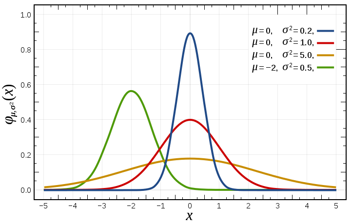
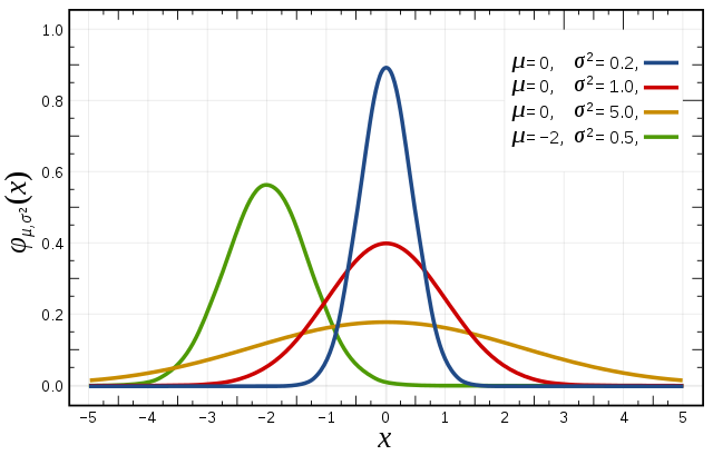
English: A selection of Normal Distribution Probability Density Functions (PDFs). Both the mean, μ, and variance, σ², are varied. The key is given on the graph. |
||
| दिनांक | |||
| स्रोत | self-made, Mathematica, Inkscape | ||
| लेखक | Inductiveload | ||
| अनुमति (इस चित्र का पुनः उपयोग करना) |
|
||
| SVG genesis | |||
| मूल कोड | R codePlot[
{
PDF[NormalDistribution[1, Sqrt[2]], x],
PDF[NormalDistribution[2, 1], x],
PDF[NormalDistribution[3, Sqrt[3]], x],
},
{x, -5, 5},
PlotRange -> All,
Axes -> False]
Data# Normal Distribution PDF
#range
x=seq(-5,5,length=200)
#plot each curve
plot(x,dnorm(x,mean=0,sd=sqrt(.2)),type="l",lwd=2,col="blue",main='Normal Distribution PDF',xlim=c(-5,5),ylim=c(0,1),xlab='X',
ylab='φμ, σ²(X)')
curve(dnorm(x,mean=0,sd=1), add=TRUE,type="l",lwd=2,col="red")
curve(dnorm(x,mean=0,sd=sqrt(5)), add=TRUE,type="l",lwd=2,col="brown")
curve(dnorm(x,mean=-2,sd=sqrt(.5)), add=TRUE,type="l",lwd=2,col="green")
Text# Normal Distribution
import numpy as np
import matplotlib.pyplot as plt
def make_gauss(N, sig, mu):
return lambda x: N/(sig * (2*np.pi)**.5) * np.e ** (-(x-mu)**2/(2 * sig**2))
def main():
ax = plt.figure().add_subplot(1,1,1)
x = np.arange(-5, 5, 0.01)
s = np.sqrt([0.2, 1, 5, 0.5])
m = [0, 0, 0, -2]
c = ['b','r','y','g']
for sig, mu, color in zip(s, m, c):
gauss = make_gauss(1, sig, mu)(x)
ax.plot(x, gauss, color, linewidth=2)
plt.xlim(-5, 5)
plt.ylim(0, 1)
plt.legend(['0.2', '1.0', '5.0', '0.5'], loc='best')
plt.show()
if __name__ == '__main__':
main()
|
चित्र का इतिहास
फ़ाइलका पुराना अवतरण देखने के लिये दिनांक/समय पर क्लिक करें।
| दिनांक/समय | थंबनेल | आकार | सदस्य | प्रतिक्रिया | |
|---|---|---|---|---|---|
| वर्तमान | 16:06, 29 अप्रैल 2016 | | 720 × 460 (63 KB) | Rayhem | Lighten background grid |
| 17:19, 22 सितंबर 2009 |  | 720 × 460 (65 KB) | Stpasha | Trying again, there seems to be a bug with previous upload… | |
| 17:15, 22 सितंबर 2009 |  | 720 × 460 (65 KB) | Stpasha | Curves are more distinguishable; numbers correctly rendered in roman style instead of italic | |
| 14:07, 27 जून 2009 |  | 720 × 460 (55 KB) | Autiwa | fichier environ 2 fois moins gros. Purgé des définitions inutiles, et avec des plots optimisés au niveau du nombre de points. | |
| 18:22, 5 सितंबर 2008 |  | 720 × 460 (109 KB) | PatríciaR | from http://tools.wikimedia.pl/~beau/imgs/ (recovering lost file) | |
| 19:09, 2 अप्रैल 2008 | कोई थंबनेल नहीं है | (109 KB) | Inductiveload | {{Information |Description=A selection of Normal Distribution Probability Density Functions (PDFs). Both the mean, ''μ'', and variance, ''σ²'', are varied. The key is given on the graph. |Source=self-made, Mathematica, Inkscape |Date=02/04/2008 |Author |
चित्र का उपयोग
निम्नलिखित पन्ने इस चित्र से जुडते हैं :
चित्र का वैश्विक उपयोग
इस चित्र का उपयोग इन दूसरे विकियों में किया जाता है:
- ar.wikipedia.org पर उपयोग
- az.wikipedia.org पर उपयोग
- be-tarask.wikipedia.org पर उपयोग
- be.wikipedia.org पर उपयोग
- bg.wikipedia.org पर उपयोग
- ca.wikipedia.org पर उपयोग
- ckb.wikipedia.org पर उपयोग
- cs.wikipedia.org पर उपयोग
- cy.wikipedia.org पर उपयोग
- de.wikipedia.org पर उपयोग
- de.wikibooks.org पर उपयोग
- de.wikiversity.org पर उपयोग
- de.wiktionary.org पर उपयोग
- en.wikipedia.org पर उपयोग
- Normal distribution
- Gaussian function
- Information geometry
- Template:Infobox probability distribution
- Template:Infobox probability distribution/doc
- User:OneThousandTwentyFour/sandbox
- Probability distribution fitting
- User:Minzastro/sandbox
- Wikipedia:Top 25 Report/September 16 to 22, 2018
- Bell-shaped function
- Template:Infobox probability distribution/sandbox
- Template:Infobox probability distribution/testcases
- User:Jlee4203/sandbox
- en.wikibooks.org पर उपयोग
- Statistics/Summary/Variance
- Probability/Important Distributions
- Statistics/Print version
- Statistics/Distributions/Normal (Gaussian)
- General Engineering Introduction/Error Analysis/Statistics Analysis
- The science of finance/Probabilities and evaluation of risks
- The science of finance/Printable version
- en.wikiquote.org पर उपयोग
- en.wikiversity.org पर उपयोग
इस चित्र के वैश्विक उपयोग की अधिक जानकारी देखें।